Pointing model run 2021/08
For this run we basically derive a new pointing model from scratch. The M1 pressure LUT were updated, derived from data of the M1 position.
For more information see sitcomtn-015.
Observations
The data for this run was taken following a similar procedure to that of Observations.
A summary of the observations, with the number of data points taken each night is shown in Observation journal. We only managed to take data on the first night of the run. The second and third night were closed due to weather.
| Night | Set | Number of observations |
|---|---|---|
| 2021/08/17 | 1 | 23 |
| 2021/08/17 | 2 | 32 |
| 2021/08/17 | 3 | 30 |
| Total | 85 |
The total number of observations in Table 2 are split into 3 type. We did 2 runs of systematic data colection (set 1 and 2) plus additional data taken when colimating the optics and/or when verifying the pointing model (set 3).
Data Analysis
The data analysis follows a similar procedure to that of Data Analysis.
EFD Data Mining
papermill -p year 2021 -p month 08 -p day 16 -p time_window 4 -p data_path /readonly/repo/main reducing_pointing_data.ipynb reducing_pointing_data/20210816_tw004.ipynb
Generating Pointing File
papermill -p pointing_data_file data/20210816/AT_point_data_20210816_tw004.pickle build_pointing_data.ipynb build_pointing_data/20210806_tw004.ipynb
Generating Pointing Model
Since we obtained 2 independent datasets, plus additional data, it is worth exploring the differences between the pointing models obtained individually.
Using dataset 1 alone we obtain the following pointing model, for a fixed set of minimum parameters;
   coeff         value    sigma

1     IA       -295.87    4.285
2     IE       -224.39    2.644
3     CA        +92.68    2.644
4     AN        +39.40    0.837
5     AW        +75.51    0.837
6     TF        -33.02    4.285

Sky RMS =   3.69
Popn SD =   4.26
For dataset 2 the same parameters yield:
   coeff         value    sigma

1     IA       -285.14    2.987
2     IE       -225.25    1.773
3     CA        +85.86    1.773
4     AN        +38.72    0.598
5     AW        +76.29    0.581
6     TF        -35.35    2.990

Sky RMS =   3.04
Popn SD =   3.37
The values of the parameters mostly agree at the 1-sigma level for both datasets. The only exception is the CA parameter which is the collimation error, e.g., the non-perpendicularity between the nominated pointing direction and the elevation axis.
Combining both datasets yields:
    coeff          value    sigma

1     IA         -289.81    2.622
2     IE         -224.83    1.585
3     CA          +88.97    1.585
4     AN          +39.09    0.520
5     AW          +76.01    0.511
6     TF          -34.18    2.623

Sky RMS =   3.51
Popn SD =   3.71
We also obtained a model with the entire dataset. Nevertheless, dataset 3 is mostly comprised of data taken while obtaining data for the hexapod lookup table, and is concentrated on two specific azimuth.
The result is:
   coeff         value    sigma

1     IA       -288.14    2.586
2     IE       -223.85    1.578
3     CA        +87.84    1.578
4     AN        +39.57    0.537
5     AW        +75.72    0.528
6     TF        -33.06    2.585

Sky RMS =   4.01
Popn SD =   4.19
Which, although has a slightly higher sky RMS, is also in agreement with the model obtained with dataset 1 and 2 combined.
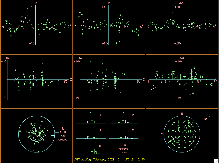
Figure 3 below shows the diagnostics plots from this model. One can notice that there are still some correlated erros, especially in the top 3 pannels, which shows;
- The “left-right” residuals plotted against azimuth.
- The elevation residuals plotted against azimuth.
- The residual az/el non-perpendicularity plotted against azimuth.

Figure 3 The “9 favorite plots for altazimuth”. This plot gathers the 9 most relevant plots with information about the pointing model fit for an altaz mount.
We attempted to fit a higher-order model to the dataset. We do obtain a slightly improved sky RMS (3.44 arcsec) but in this case, we still observe some correlated errors on the diagnostic plots. In order to avoid overfitting, we decided to keep the lower order fit shown above.